


Start from: Your Excel file, open
Open your file
- Launch Excel.
- Open the file containing the data you want to filter.
- Select a cell in your table.
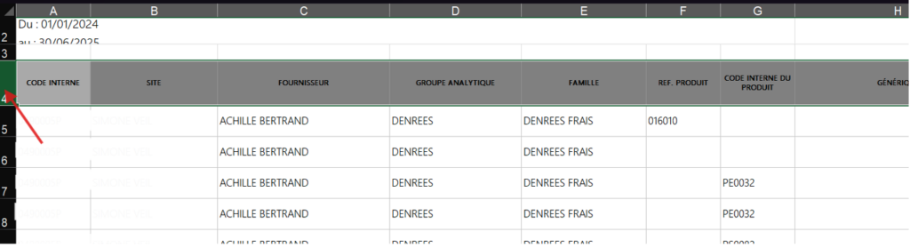
Enable the filter
There are two methods. Use whichever suits you.
Method 1: from the Home tab
- Select the Home tab at the top of the window.
- Select Sort & Filter, in the Editing group at the right of the ribbon.
- Select Filter.
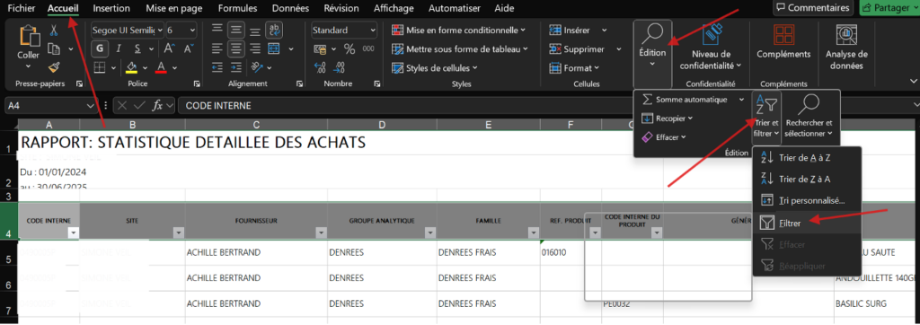
Note: You can also use the keyboard shortcut Ctrl + Shift + L.
Method 2: from the Data tab
- Select the Data tab at the top of the window.
- Select the Filter icon, shaped like a funnel.
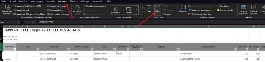
An arrow appears in each column header.

Use the filter
- Select the arrow in the column you want to filter.
- Clear (Select All).
- Select only the values you want to display.
- Select OK.
Your table now displays only the rows matching your selection..
